Signal Detection Theory is a widely used framework for understanding decisions by distinguishing between response bias and true discriminability in various psychological domains. Manual calculation approaches to estimating SDT models’ parameters, while commonly used, can be cumbersome and limited. In this tutorial I connect SDT to regression models that researchers are already familiar with in order to bring the flexibility of modern regression techniques to modeling of SDT data. I begin with a glance at SDT’s fundamentals, and then show how to manually calculate basic SDT parameters. In the bulk of the tutorial, I show step-by-step implementations of various SDT models using the brms R package. I progress from analyses of binary Yes/No tasks to rating task models with multilevel structures, unequal variances, and mixtures. Throughout, I highlight benefits of the regression-based approach, such as dealing with missing data, multilevel structures, and quantifying uncertainty. By framing SDT models as regressions, researchers gain access to a powerful set of flexible tools while maintaining the conceptual clarity that makes SDT valuable. A regression-based approach not only simplifies SDT analyses but also extends SDT’s utility through flexible parameter estimation with uncertainty measures and the ability to incorporate predictors at multiple levels of analysis.
Signal Detection Theory (SDT) is a framework for studying, understanding, and modeling a wide range of psychological phenomena (Green and Swets 1966). Its origins are in the psychophysical study of perception, but it has since been used to understand memory, decision making, and other domains. So what is SDT?
“Detection theory entered psychology as a way to explain detection experiments, in which weak visual or auditory signals must be distinguished from a ‘noisy’ background.”(Macmillan and Creelman 2005, xiii)
To unpack this definition, consider a recognition memory experiment where participants view a series of images, some of which they have not seen before (new items) and some of which they have seen before (old items). For each item, participants decide whether they have seen the item before (and thus give an “old” response) or not (a “new” response).
A straightforward analysis of data from this experiment focuses on accuracy: What percentage of items participants correctly classified as old or new? Such analyses of accuracy, however, are suboptimal because they conflate two critical factors, fundamental to SDT, that plausibly underlie participants’ responses: Response bias (commonly termed c for criterion) and the ability to discriminate old from new items (commonly termed d’ for discriminability). Through directly modeling these two processes, SDT has repeatedly been shown to explain data better than models implied by analyses of accuracy (Macmillan and Creelman 2005, 13; Kellen et al. 2021). Why?
In this hypothetical experiment, participants might respond “old” for (at least) two reasons: A tendency to respond “old”, and an underlying ability to discriminate previously seen items from new items. The conceptual basis of SDT (keeping with a memory task example) is that each stimulus elicits some experience of “familiarity” (commonly termed signal strength or evidence). Because of noise in the environment and perceptual, cognitive, and other information processors involved, even for a fixed stimulus the resulting evidence is not constant but instead varies from trial to trial.
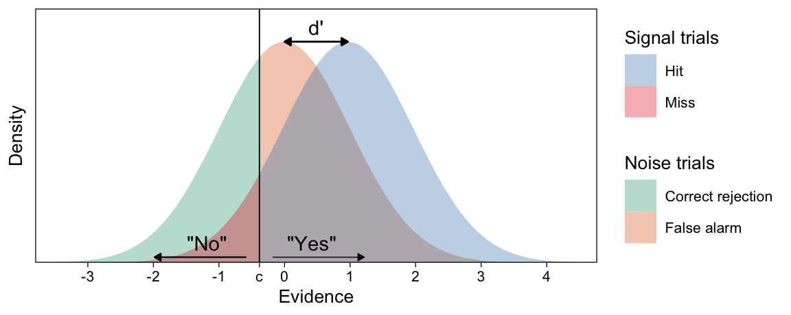
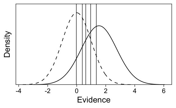
Figure 1: Illustration of subjective evidence distributions postulated by Signal Detection Theory. Each stimulus presentation elicits a degree of evidence, which is assumed to be normally distributed as a sum of many unknown sources of noise in the information processing flow from stimulus to consciousness. On noise trials (left; e.g. new items in a memory experiment), the evidence distribution is centered on zero. On signal trials (right; e.g. old items) the distribution has some positive mean if the participant can—on average—distinguish the signal from noise. The vertical line illustrates the decision criterion c which the evidence must exceed for a participant to decide that the trial contained a signal. The distance between the two distributions’ means indicates discriminability d’.
The participants then decide, based on whether current evidence exceeds their criterion, whether they’ve seen the stimulus previously (“old”) or not (“new”). Some individuals might have a liberal bias and report “old” on trials with even modest degrees of evidence. Others might be conservative and require a greater degree of evidence before deciding they’ve seen the stimulus before. The decision process posited by SDT, based on subjective evidence and thresholds, is visualized in Figure 1.
Since the introduction of SDT in studies on perception, and its later widespread adoption in e.g. memory research, the conceptual framework and analytic machinery has been applied in a broad range of areas. For example, in one study, we showed participants photographs of individuals who were injected with a bacterial endotoxin or not, and participants’ task was to detect whether the individual was ill or not (Leeuwen et al. 2024). In another, participants viewed videos of individuals that were either lying or not, and their task was to determine whether the individual was lying or not (Zloteanu and Vuorre 2024). The key to SDT’s success in such a wide variety of domains lies in its applicability even in the absence of information about the kinds of cues that inform people’s decisions:
“A full understanding of the decision process […] is difficult, if not impossible. The decisions depend on many particulars: what the decider knows, his or her expectations and beliefs, how later information affects the interpretation of the original observations, and the like. An understanding of much domain-specific knowledge is needed […]. Fortunately, much can be said about the decision process without going into these details. Some characteristics of a yes-no decision transcend the particular situation in which it is made. The theory discussed here treats these common elements. This theory, known generally as signal-detection theory, is one of the greatest successes of mathematical psychology.”(Wickens 2001, 4, emphasis added)
Our conceptual treatment of SDT, for the purposes of an applied tutorial, was necessarily brief. Readers interested in more complete treatments should consult books such as Wickens (2001), Macmillan and Creelman (2005), or Green and Swets (1966). An accessible article with computational details is Stanislaw and Todorov (1999).
Current work: Estimating SDT models with regression
While SDT posits latent probability distributions as the basis for decision making, it is also widely applicable as a relatively theory-free analytic framework that simply allows separating response biases from latent abilities, as suggested by the examples above. It is therefore often considered a standard tool in any behavioral scientist’s toolkit. Subsequently, software packages for calculating SDT metrics and tutorials illustrating their uses are common (Lee 2008; Paulewicz and Blaut 2020; Cohen et al. 2021).
In this tutorial, I take a different approach: Much of a behavioral scientist’s quantitative training focuses on the General(ized) Linear Model (regression) framework. It is therefore useful to draw a direct connection between this class of common cognitive models (SDT) to tools that researchers already know (GLM) (see also DeCarlo 1998, 2010; Decarlo 2003).
Moreover, rather than focusing on computational methods for obtaining point estimates of SDT metrics, as is commonly done (e.g. Stanislaw and Todorov 1999), using the regression framework to estimate them allows quantifying degrees of uncertainty (e.g. standard errors) in the resulting estimates. Finally, by establishing SDT models as regressions, we gain all the benefits of regression, such as including categorical and continuous within- and between-subject predictors, using multilevel structures for crossed item and subject effects (Rouder and Lu 2005; Rouder et al. 2007), model comparison, and support of established software packages.
We first focus on analyses of “Yes/No” tasks, where participants’ task is to provide a binary “Yes” or “No” response to a stimulus that either does or does not contain the “signal” that participants attempt to detect. In the ongoing memory example, previously seen (old) items are the signal stimuli, and new items the noise stimuli. I first illustrate how to calculate SDT metrics “manually” using R (R Core Team 2025). Then, I show the corresponding R syntax for estimating the SDT model as a regression for an individual subject. We then discuss two methods for obtaining estimates of population-level SDT parameters by first aggregating subject-specific estimates, and then by estimating multiple subjects’ SDT parameters simultaneously with a multilevel model.
After discussing analyses of the basic Yes/No task, I move to rating tasks where participants provide ordinal responses that indicate their confidence in whether a stimulus contained the signal or not. These rating data allow for richer inference of participant behavior and decision making processes. Correspondingly, after showing how to estimate basic SDT models of rating data with GLMMs, I illustrate more advanced models that include unequal variances and mixtures.
Throughout, I assume readers are familiar with regression models. I refer those in need of a refresher to texts such as Gelman et al. (2020), McElreath (2020), or Çetinkaya-Rundel and Hardin (2024). I implement analyses in the Bayesian framework due to its flexibility, computational robustness, and conceptual clarity. For reasons of brevity I provide minimal explanations of this framework; interested readers should consult standard texts such as Kruschke (2014), McElreath (2020), and Gelman et al. (2013). Accessible introductory articles are, for example, Kruschke and Liddell (2017b) and Kruschke and Liddell (2017a).
Finally, I show additional benefits of estimating SDT models with regression. For one, prior distributions and multilevel models deal elegantly with edge cases where participants have missing data (e.g. no false alarms). Moreover, the estimated parameters seamlessly inform other common SDT metrics, such as Receiver Operating Characteristic (ROC) curves, all of which retain and allow representing the estimation uncertainty associated with the underlying parameters.
SDT analysis of Yes/No data
The tasks outlined above are typically called “Yes/No” experiments, because the participant’s task is to provide a binary “Yes” or “No” response to a stimulus that either does or does not contain the “signal” that participants attempt to detect. In the ongoing memory example, previously seen (old) items are the signal stimuli, and new items the noise stimuli. In this tutorial, we first focus on analyses of data from Yes/No tasks.
Example Yes/No task and data
To illustrate the most commonly used SDT model, we examine data from the control condition of Experiment 2 in Koen et al. (2013): 48 subjects studied a list of 200 words for 1.5s each. After a filler task, participants were tested with 200 new and 200 old words. In the test phase, participants rated their confidence in whether each word was new or old with a 6-point Likert item (1: “sure new”, 2: “maybe new”, 3: “guess new”, 4: “guess old”, 5: “maybe old”, 6: “sure old”). This data set is included in the R package MPTinR (Singmann and Kellen 2013).
For the purposes of the first part of this tutorial, and following the authors’ first analysis (Table 1 in Koen et al. (2013)), we first bin the rating responses to binary “new” (1-3) and “old” (4-6) responses. The resulting data (Table 1) is then typical of Yes/No tasks.
Code
# Koen 2013data(roc6, package ="MPTinR")dat <-tibble(roc6) |>filter(exp =="Koen-2013_immediate") |>separate(id, c("id", "exp2"), sep =":") |>select(-exp, -exp2) |>pivot_longer(-id, values_to ="n") |>separate(name, into =c("stimulus", "response")) |>mutate(pid =fct_inorder(factor(id)),stimulus =factor( stimulus,levels =c("NEW", "OLD"),labels =c("New", "Old") ),response =factor( response,levels =c("3new", "2new", "1new", "1old", "2old", "3old"),labels =1:6 ) |>as.integer(),.keep ="unused",.before =1 )# Save ordinal data for part 2dat2 <- dat# Convert to binary responses for part 1dat <- dat |>mutate(response =if_else(response %in%1:3, "New", "Old") |>factor() )# Unaggregate and add trial number to clarify data structuredat <-uncount(dat, n) |>mutate(trial =1:n(), .by = pid, .after =1)
Code
set.seed(11)slice_sample(dat, n =4) |>arrange(pid, trial) |>tt()
Table 1: Four rows of example recognition memory data from Koen et al. (2013).
pid
trial
stimulus
response
1
34
Old
New
3
96
Old
Old
4
21
Old
New
6
286
New
Old
Calculating SDT parameters
It is immediately clear how to calculate a participant’s overall accuracy from data in Table 1: Add up the trials where stimulus and response are identical, and divide the sum by the total number of trials. Calculating SDT parameters, to which we now turn, is not much more involved (Stanislaw and Todorov 1999).
First, responses from a Yes/No task are divided into four categories: hits (responding “old” to old items), misses (responding “new” to old items), false alarms (responding “old” to new items), and correct rejections (responding “new” to new items). We then calculate hit and false alarm rates by aggregating the response categories, z-score the rates, and either add (to calculate response bias) or subtract (to calculate sensitivity) these z-scores. I first show how to classify trials with R in Listing 1.
Listing 1: Classifying Yes/No trials into hits, misses, false alarms, and correct rejections using the case_when() function from the dplyr R package.
After classifying trials, we aggregate participants’ data to hit (hits / (hits + misses)) and false alarm rates (false alarms / (false alarms + correct rejections); see Figure 1) in Listing 2, where we also pivot the data to one row per participant (Table 2).
Listing 2: Classifying Yes/No experiment trials into hits, misses, false alarms, and correct rejections using the case_when() function from the dplyr R package.
Table 2: Aggregated task behavior of each participant.
pid
cr
fa
hit
miss
hr
fr
1
110
40
116
34
0.77
0.27
2
100
50
119
31
0.79
0.33
3
118
32
126
24
0.84
0.21
4
104
46
117
33
0.78
0.31
We can then calculate the two SDT parameters from the hit and false alarm rates: The decision criterion c and discriminability d’. d’ is calculated as the difference of the normal distribution scores, also commonly referred to as “z-scores”, of the hit and false alarm rates (Stanislaw and Todorov 1999):
\[
d' = \Phi^{-1}(HR) - \Phi^{-1}(FAR)
\tag{1}\]
\(\Phi\) is the normal distribution function, and is used to convert z scores into probabilities. It is available in R as pnorm(). \(\Phi^{-1}\), the normal quantile function (available in R as qnorm()), converts proportions into z scores.
But why do we use a normal distribution? Recall from above that SDT posits that each stimulus leads to a subjective (or “latent”) value of evidence. This evidence is not fixed by the stimulus but varies from trial to trial because of noise in the system perceiving the stimulus. We do not know what the myriad sources of this variability might be, so the normal distribution that results from the sum of many independent variations, is a natural choice. Note that other distributions, although rarely used, are possible (DeCarlo 1998).
The response criterion c is calculated as:
\[
c = -\frac{\Phi^{-1}(HR) + \Phi^{-1}(FAR)}{2}
\tag{2}\]
It is important to note that most treatments use a minus sign in the calculation of c(e.g. Stanislaw and Todorov 1999). This means that negative values of c indicate a “liberal” bias toward responding “yes”, and positive values of c indicate a “conservative” tendency toward responding “no” (see Figure 2). An alternative parameterization omits the negative sign, in which case positive values of c indicate a (“liberal”) bias toward responding “yes”, and negative values of c indicate a (“conservative”) bias toward responding “no”.
Listing 3: Calculating z-scored hit and false alarm rates and the SDT parameters c and d’.
I z-score the hit and false alarm rates and then calculate each participant’s c and d’ from the z-scores in Listing 3. The resulting data table is shown in Table 3.
Table 3: Four subjects’ SDT parameters and the quantities used to calculate them.
pid
hr
fr
zhr
zfr
crit
dprime
1
0.77
0.27
0.75
-0.62
-0.06
1.37
2
0.79
0.33
0.82
-0.43
-0.19
1.25
3
0.84
0.21
0.99
-0.79
-0.10
1.79
4
0.78
0.31
0.77
-0.51
-0.13
1.28
(As a side note, c is only one of many bias measures. For example, early researchers on SDT, such as J. C. R. Licklider—who incidentally also laid the groundwork for the modern Internet—favored a likelihood ratio measure (Licklider 1959; Macmillan and Creelman 2005, 31–36).)
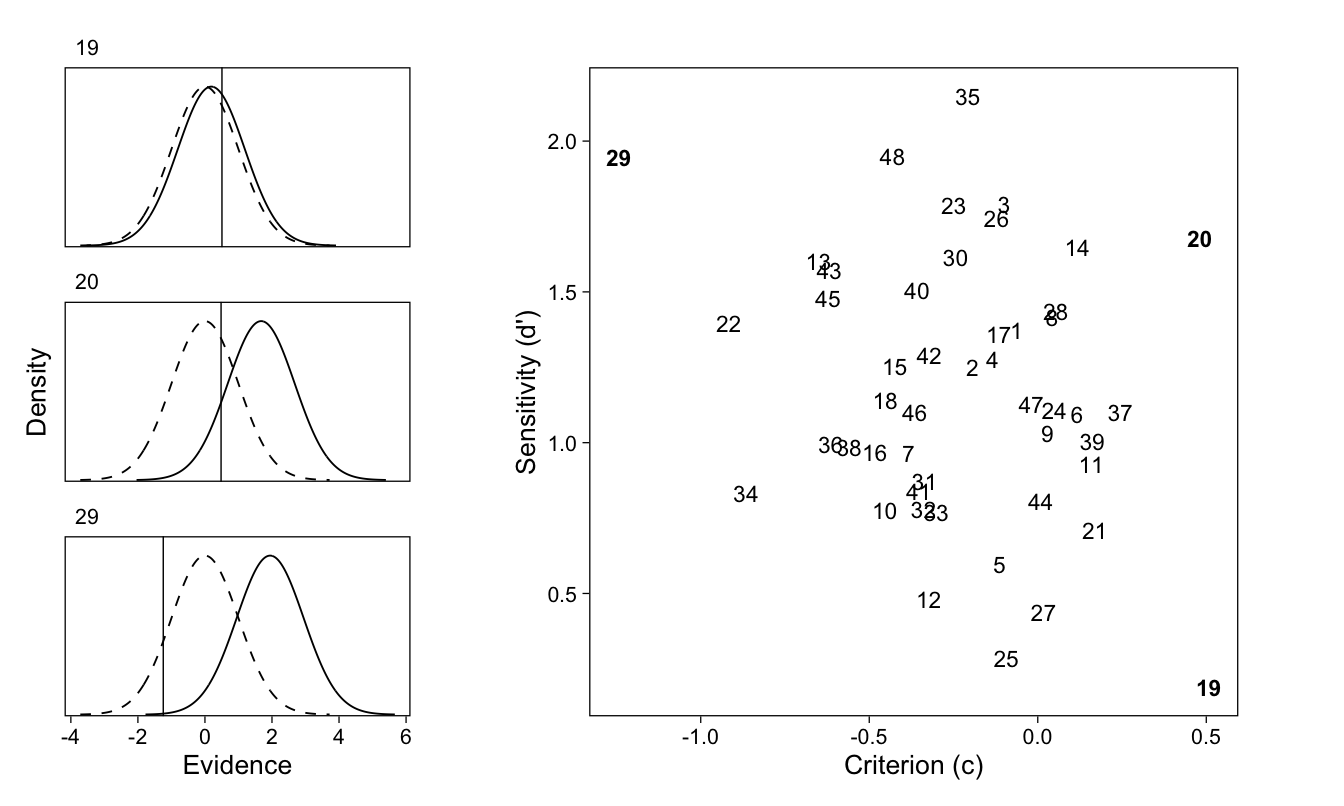
The sdt data frame (Table 3) now has every participant’s d’ and c, and the quantities that went into calculating them. I show three participants’ implied SDT models, and all participants’ SDT parameters, in Figure 2.
Figure 2: Left. The signal detection model for three participants. The two curves are the noise (dashed) and signal distributions (solid); the vertical line represents the response criterion c. d’ is the distance between the two distributions’ means. Of these three participants, 29 has the lowest c and therefore the most liberal response bias. Participant 19 has the smallest d’ and therefore the worst ability to discriminate between new and old items. Right. Scatterplot of all participants’ criteria and d’, with the three participants shown in the left panel highlighted in bold font.
Estimating SDT parameters with regression
We have now “manully” calculated, rather than statistically estimated, participants’ SDT parameters. While standard practice, this approach has at least two potential downsides. First, we have not quantified our uncertainty in the parameters. For example, were we interested in a statistical comparison of participant 19’s and 29’s criteria, we could only report a point estimate of this difference.
Second, any further questions—estimating (differences in) population means, for example—would require additional models of these point estimates. These further models would ignore the uncertainty inherent in the participant-specific parameters. This point may not matter for perfectly balanced designs, but would be especially important when participants complete different numbers of trials or have missing data.
Moreover, while it is pedagogically useful to go through these calculations, there might also be related downsides: These quantities are naturally estimated in common regression models, and by not making that connection explicit we are not contributing as effectively to further quantitative learning. Because researchers are typically already familiar with regression techniques, using those instead of manual calculations may prove useful in practice as well (Decarlo 2003).
Therefore, we now move to the main topic of this tutorial: Estimating SDT models using Generalized Linear Models (GLM).
Coding categorical variables
We begin by considering the raw data in Table 1. Because the data contains categorical variables, it is first important to understand how a model might use them. In R, this specification is done via “contrasts” (such as dummy variables, contrast codes, etc) that code them into numerical values when used in models.
When binary variables are modeled in R (either as outcomes or predictors), R by default will assign them treatment codes (also known as dummy variables). Therefore stimulus and response would be coded as “New”: 0 and “Old”: 1 (from their alphabetical order). For reasons visible to some readers in Equation 2 and further elaborated below, we instead sum-to-zero-code stimulus as “New”: -0.5 and “Old”: 0.5 (Table 4). This will ensure that our model’s intercept will be “halfway between” the (z-scored) hit and false alarm rates (now take another look at Equation 2). I specify this coding scheme in Listing 4.
Listing 4: Creating sum to zero contrast codes for the stimulus variable.
Table 4: Numerical contrast codes of categorical variables when modeled.
Contrast code
Data value
stimulus
response
New
-0.50
0
Old
0.50
1
Specifying the model
Now that we have prepared our data, we proceed to specifying our regression model. We first consider this model for one participant. We model responses r (“No”: 0, “Yes”: 1) at row i as Bernoulli distributed with probability \(p_i\) that \(r_i = 1\) (line 1 below). (Bernoulli distribution is the binomial distribution for binary responses.)
Because probabilities have lower and upper limits at 0 and 1, we model p through a link function. A common choice for a link function for models of binary data is the logistic, leading to the familiar logistic regression model. However, we use the probit link function \(\Phi\) which maps the unbounded continuous linear combination of the predictors to probabilities (line 2 above).
Given this parameterization, the intercept of the model (\(\beta_0\)) will indicate the z-scored probability of responding “old” when all predictors are zero (see Listing 4). When stimulus, our predictor, is “sum-to-zero” coded as we have done above, the intercept corresponds to -c (see Equation 2). The slope of the model (\(\beta_1\)) is the difference in z-scored probabilities of saying “old” between old and new items, and therefore \(d' = \beta_1\) (see Equation 1). For a more complete treatment of the connection between SDT models and GLM, see DeCarlo (1998).
Estimating the model
We now have a variety of software options for estimating the GLM. For this simple model, we could use base R’s glm(). Here, we use the Bayesian regression modeling R package brms(Bürkner 2017), because its model formula syntax extends seamlessly to more complicated models that we will discuss later. We can estimate the GLM with brms’s brm() function by providing as arguments a model formula in brms syntax (identical to base R model syntax for simple models), an outcome distribution with a link function, and a data frame.
brms’s model syntax uses variable names from the data. In Listing 5, we regress the binary response outcome on the binary stimulus predictor (response ~ stimulus). We then specify that outcomes are bernoulli distributed with a probit link function with family = bernoulli(link="probit"). We will only model the first participant’s data, and therefore specify the data with data = filter(dat, pid==1).
The brm() function also allows specifying prior distributions on the parameters, but for this introductory discussion we omit discussion of priors. Finally, we specify file to save the estimated model to a file so that we don’t have to re-estimate the model whenever we restart R.
Listing 5: Fitting the SDT model as a GLM with the brm() function
# I also fit the model separately to all participantspath <-"cache/brm-glm-all.rds"if (!file.exists(path)) { fit_glm_all <- dat |>nest(.by = pid) |>summarise(fit =map( data,~update( fit_glm,newdata = .x,recompile =FALSE ) ),.by = pid )saveRDS(fit_glm_all, path)} else { fit_glm_all <-readRDS(path)}
The estimated model is saved in fit, whose summary() method returns a numerical summary of the estimated parameters along with some information and diagnostics about the model:
The regression parameters (Intercept (\(-c = \beta_0\)) and stimulus1 (\(d' = \beta_1\))) are described in the “Regression Coefficients” table in the above output. Estimate reports the posterior means, which are comparable to maximum likelihood point estimates. Est.Error reports the posterior standard deviations, which are comparable to standard errors. The estimated parameters’ means match the point estimates we calculated by hand (see Table 3), but note the reversed sign of c. The next two columns report the parameter’s 95% Credible Intervals (CIs). Finally, the Rhat and _ESS values provide diagnostic information (convergence and effective posterior sample size, respectively) about the Bayesian estimation procedure. The former should be close to 1.00, and the latter as large as possible. We do not consider these metrics further, but see e.g. Gelman et al. (2013).
Interpreting the model
We read in the above output that the model intercept, corresponding to -c, has a positive posterior mean, but its CI considerably overlaps zero. Therefore, this participant is not strongly biased in favor of responding either “Yes” or “No”. The slope coefficient stimulus1, corresponding to d’, is positive and indicates that the latent evidence distribution of signal trials for this participant is ~1.4 z-scores greater than the noise distribution: The participant has good discriminability and is able to tell old stimuli from new.
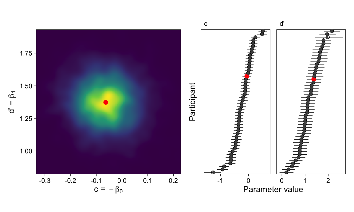
We now return to the two shortcomings of manually calculating SDT parameters alluded to above. First, the model assigns credibility to a range of parameter values (the CI), instead of returning only the most likely value (the posterior mean). I illustrate these degrees of certainty in the left panel of Figure 3. This figure is a smoothed bivariate density of the scatterplot of posterior samples of \(p(\beta_0, \beta_1)\), and indicates more credible SDT parameter values in lighter yellow hues. The point estimate shown in red is a poor representation of this more complete picture.
Figure 3: SDT parameters as estimated with a Generalized Linear Model. Left. The (approximate) joint posterior density of subject 1’s SDT parameters. Lighter hues indicate higher posterior density and therefore parameter values in which we are more confident. The red dot indicates the manually calculated point estimate of c and d’. Right. Posterior means and 95%CIs of all participants’ parameters (empty circles and intervals) along with manually calculated point estimates (filled circles). The two are in perfect agreement.
Second, consider the bottom and top points in the c column of Figure 3. All we could say based on the point estimates is that the top participant has a far more positive (conservative) criterion than the bottom participant. However, the bayesian estimates would allow directly testing that difference, by virtue of retaining uncertainty in the parameter estimates. Finally, notice how straightforward it was to estimate the SDT parameters with regression: Instead of multiple lines of data wrangling and calculation, the regression model directly returns SDT parameters from the raw data.
SDT for multiple participants
We have now estimated the SDT model’s parameters for one subject’s data using two methods: Calculating point estimates manually and estimating them with a GLM. The main difference between these methods is that modeling provided estimates of uncertainty in the parameters, whereas the manual calculation did not. This point leads us directly to multilevel models (Rouder and Lu 2005; Rouder et al. 2007; Gelman and Hill 2007), which we discuss next.
Researchers are usually not primarily interested in the specific subjects that happened to participate in their experiment. Instead the population of potential subjects is the target of inference. Therefore, we are unsatisfied with parameters which describe only the individuals in our sample: The final statistical model should have parameters that estimate features of the population of interest.
Broadly, there are two methods for obtaining these population-level parameters. The most common method is to aggregate manually calculated subject-specific point estimates of d’ and c to their sample means and standard deviations. From these, we can calculate standard errors, t-tests, confidence intervals, and so on. The second method involves fitting one model simultaneously to all participants’ data.
Estimating by summarizing subjects’ point estimates
Above we calculated d’ and c for every participant in the sample. We can therefore calculate sample means and standard errors for both parameters using these individual-specific values. I show one way to do this aggregation in R using summarise() from the dplyr package in Listing 6.
The sample means are estimates of the population means, and the sample standard deviations divided by square root of the number of subjects are standard deviations of the means’ sampling distributions, the standard errors. Note that this method involves calculating point estimates of unknown parameters (the subject-specifc estimates), and then summarizing these parameters with additional models. In other words, we first fit N models with P parameters each (N = number of subjects, P = 2 parameters), and then P more models to summarise the subject-specific models.
Multilevel model
Another method is to build a multilevel model that simultaneously estimates subject-specific and population-level parameters (Gelman and Hill 2007; McElreath 2020). Rouder and Lu (2005) and Rouder et al. (2007) discuss multilevel models in the context of Signal Detection Theory. Multilevel models are variously also known as hierarchical, mixed, random-effect, and Generalized (Linear) Mixed Models (GLMMs).
This model is identical to the GLM in Equation 3, but now the subject-specific d’s and -cs are modeled as draws from a multivariate normal distribution, whose parameters describe the population. We subscript subjects’ parameters \(\gamma\) with j, rows in data with i, and write the model as:
The responses \(r_{ij}\) are 0 if participant j responded “new” on trial i and 1 if they responded “old”. The probability of an “old” response on row i for subject j is \(p_{ij}\) (line 1 in Equation 4). We then write a linear model on the p’s z-scores (\(\Phi\), line 2). The subject-specific intercepts (recall, \(-\gamma_{0j} = c_j\)) and slopes (\(\gamma_{1j} = d'_j\)) are now deviations from population-level parameters \(\beta\), which can be interpreted as parameters “for the average person” (Bolger and Laurenceau 2013).
These subject-specific deviations are modeled as draws from a multivariate normal distribution, whose covariance matrix \(\Sigma\) contains the (co)variances of the parameters in the population (line 3). The software we use instead estimates standard deviations and correlations, and so the covariance matrix is constructed on line 4. The standard deviations \(\tau\) describe the between-person heterogeneities in the population. The correlation term \(\rho\) describes the relationship between d’ and c: Are people with a higher d’ more likely to have a higher c? This model is therefore more informative than running multiple separate GLMs, because it allows examining parameters’ heterogeneity in the population (e.g. Vuorre et al. 2024).
The brms syntax for this model is very similar to the one-subject model. We have five population-level parameters to estimate (\(\beta, \tau, \rho\)). The intercept and slope describe the means: In R and brms modeling syntax, an intercept is indicated with 1 (it is automatically included, so I omit it), and slope of a variable by including that variable’s name in the data.
However, we also have three (co)variance parameters to estimate. To include subject-specific parameters (recall, subjects are indexed by pid in the data frame), and therefore their (co)variance parameters, we expand the formula to response ~ stimulus + (stimulus | pid). Otherwise, the call to brm() is the same as with the GLM above:
However, before proceeding, we introduce a computational shortcut. As the number of trials and participants increases, data in long format (such as dat shown in Table 1) quickly grows in size. Because of how Bayesian models are estimated, larger data and more complex models increase the model estimation time. We therefore estimate exactly the same model, but on data that is aggregated to counts of unique response-predictor combinations to speed up the estimation process. We do this in Listing 7, where we aggregate the raw data (with 14400 rows) to a table of pid-stimulus-response counts (indicated by n in the data table that now has 192 rows). We can then reap the speed benefits of this data aggregation by using weights(n) to indicate how much weight to give to observation.
Listing 7: Fitting the SDT model for multiple participants as a GLMM with brm().
The Regression Coefficients in the output below are -c (Intercept = \(\beta_0\)) and d’ (stimulus1 = \(\beta_1\)) for the average person. Recall that we are looking at numerical summaries of (random samples from) the parameters’ posterior distributions: Estimate is the posterior mean, Est.Error the posterior standard deviations, and l-95% CI and u-95% CI the limits of the 95%CI.
Code
# Omit MCMC info in brmsfit.summary.summary <-function(x) { out <-summary(x) out$random$pid <- out$random$pid[, 1:4] out$fixed <- out$fixed[, 1:4] out$spec_pars <- out$spec_pars[, 1:4] out}.summary(fit_glmm)
 Family: bernoulli
  Links: mu = probit
Formula: response | weights(n) ~ stimulus + (stimulus | pid)
   Data: dat_agg (Number of observations: 192)

Multilevel Hyperparameters:
~pid (Number of levels: 48)
                         Estimate Est.Error l-95% CI u-95% CI
sd(Intercept)                0.34      0.04     0.27     0.42
sd(stimulus1)                0.42      0.05     0.33     0.53
cor(Intercept,stimulus1)     0.20      0.15    -0.11     0.48

Regression Coefficients:
          Estimate Est.Error l-95% CI u-95% CI
Intercept     0.22      0.05     0.12     0.33
stimulus1     1.17      0.07     1.04     1.29
These estimates tell us that the average person in the population from which our sample was drawn has a somewhat liberal response bias and good ability to discriminate old from new items. To clarify the correspondence between the two estimation methods, we can compare these population-level parameters of this model to the sample summary statistics we calculated above. The posterior means map to the calculated means, and the posterior standard deviations match the calculated standard errors (Table 5). I also visualize these estimates in Figure 4.
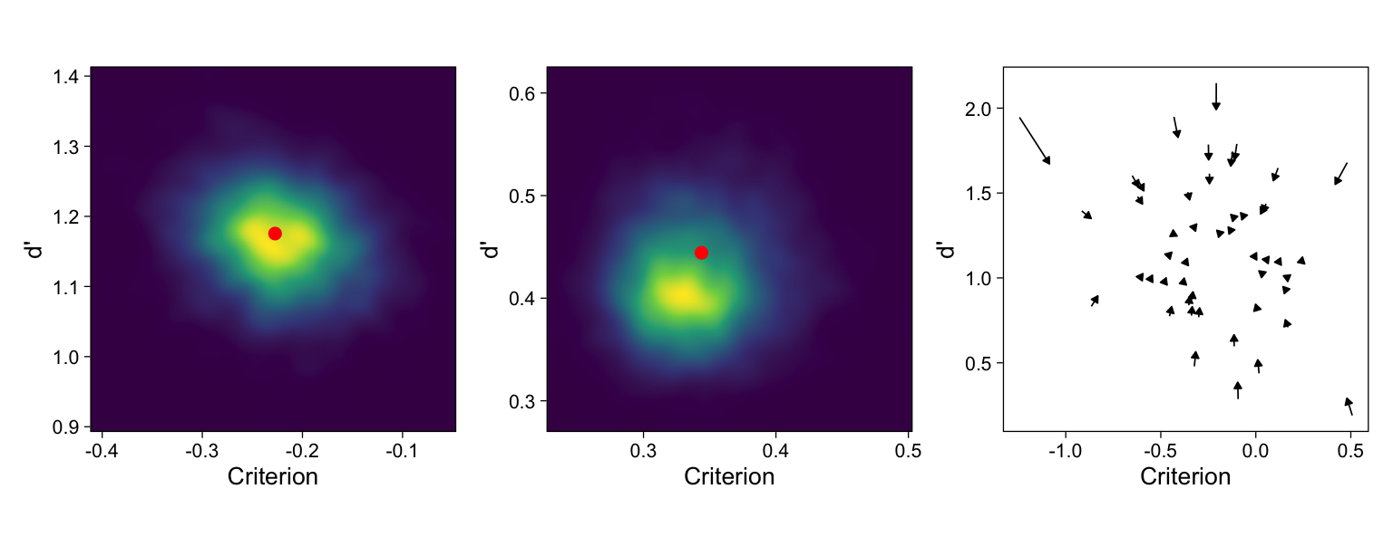
However, the GLMM also returns estimates of the parameters’ (co)variation in the population. Notice that we also calculated the sample standard deviations, but we have no estimates of uncertainty in those point estimates (Table 5). The GLMM, on the other hand, provides full posterior distributions for these parameters. The heterogeneity parameters are reported in the Multilevel Hyperparameters section, above. We find that the criteria are positively correlated with d’s. The two standard deviations are visualized in the middle panel of Figure 4.
Figure 4: Left. The (approximate) joint posterior density of the average d’ and criterion. Lighter values indicate higher posterior probability. Middle. The (approximate) joint posterior density of the standard deviations of d’ and criterion in the population. In both panels, the red dot indicates sample statistics. Right. Subject-specific d’s and criteria as given by the independent models (arrow origins), and as estimated by the hierarchical model (arrow tips). The hierarchical model shrinks the estimated parameters toward the population means. This shrinkage is greater for more extreme parameter values: Each subject-specific parameter is a compromise between that subject’s data, and other subjects in the sample.
It is evident in Figure 4 that the sample means approximately match the posterior mean population means, but less so for the standard deviations, whose sample statistics are not at the peak of the standard deviations’ posterior distribution. By ignoring the uncertainty in the subject-specific parameters, the ‘manual calculation’ method has over-estimated the heterogeneity of d’ and c in the population, in comparison to the GLMM which takes the subject-specific parameters’ uncertainty into account.
This deviation has further implications, revealed by investigating the two methods’ estimates of the subject-specific parameters. Recall that the manual calculation method involved estimating (the point estimates of) a separate model for each participant. A hierarchical model considers all participants’ data simultaneously, and the estimates are allowed to inform each other via a shared prior distribution. This “partial pooling” of information (Gelman and Hill 2007) reduces overfitting and thereby returns estimates with better predictive performance (Efron and Morris 1977). The subject-specific effects are pulled toward their means, an effect that is most visible for participants with most extreme values (right panel of Figure 4).
SDT analysis of rating data
Until now, we have considered analyses of a detection task where stimuli were either old or new, and participants provided binary “old” and “new” responses. We now turn to the Rating task where participants instead rate their degree of confidence that the stimulus was old or new.
Example rating task and data
This, as mentioned above, is exactly what subjects in Koen et al. (2013) did: On each trial, subjects responded with a 6-point Likert item indicating their confidence in the item being new or old (1: “sure new”, 2: “maybe new”, 3: “guess new”, 4: “guess old”, 5: “maybe old”, 6: “sure old”). I show these data in Table 6.
Table 6: Aggregated example data from subject 1 in the control condition of Koen et al. (2013), Experiment 2. First and last two rows are shown for brevity.
pid
stimulus
response
n
1
Old
1
15
1
Old
2
11
...
...
...
...
1
New
5
10
1
New
6
15
A common and plausible interpretation of these data is that participants use a set of criteria, such that greater evidence is required for greater numerical responses. That is, there will be different criteria for responding “definitely new”, “maybe new”, and so forth. Generally, such data is commonly analyzed with models that assume a continuous (usually normally distributed) outcome. However, this practice can lead to problems when data isn’t well-behaved, and therefore models that appropriately account for the responses’ ordinal nature are recommended (Liddell and Kruschke 2018). An accessible introduction to such ordinal models can be found in Bürkner and Vuorre (2019), and Chapter 12.3 of McElreath (2020).
Above, we noted that a GLM with a Bernoulli response function and probit link function is a regression formulation of the basic SDT model of Yes/No data. Similarly, one class of ordinal models, called the cumulative model in Bürkner and Vuorre (2019), provides a regression formulation of SDT models for data from a Rating task (see also DeCarlo 1998; Decarlo 2003).
Model for one subject
For rating data, the SDT model is very similar to the one for Yes/No task data, but now includes multiple intercepts, commonly referred to as thresholds. These thresholds index criteria that subjects use to split their internal experiences (evidence) to the different response categories, and therefore conceptually correspond to c. For k response options, we need \(k - 1\) thresholds. The criteria are ordered: People should be more likely to respond “sure old” rather than “maybe old” when evidence (memory strength) is greater. To connect with the ongoing, we label these thresholds as \(c_k\) (\(\tau_k\) in Bürkner and Vuorre (2019); \(\alpha_k\) or \(\kappa_k\) in McElreath (2020), Chapter 12.3.) We then write the probability of a response r being in category k in Equation 5.
We can consider Equation 5 as a somewhat convoluted link function, after which we specify a regression model on the linear predictor \(\eta\):
\[
\eta_i = \beta_1s_i
\tag{6}\]
Note that we conspicuously omitted an intercept in the linear model (Equation 6), because the intercepts are already included as thresholds in Equation 5: The cumulative model estimates intercepts (\(c_k\)) that partition the latent evidence distribution into response categories (k), and a slope parameter that indexes the distance between the noise and signal distribution’s means. To connect with the SDT model for Yes/No data, we label the slope (\(\beta_1\)) again as d’. The brms syntax for estimating this model with participant 1’s data is shown in Listing 8.
Listing 8: Estimating one participant’s rating data with a cumulative model.
Note that the only change from the Bernoulli model of Yes/No data (Listing 5) is that we now used family = cumulative(), and the actual rating data (dat2). In addition, we have not sum-to-zero coded the stimulus predictor for this model. The model’s posterior distribution is summarised below:
Code
summary(fit_evsdt1)
 Family: cumulative
  Links: mu = probit
Formula: response | weights(n) ~ stimulus
   Data: filter(dat2, pid == 1) (Number of observations: 12)

Regression Coefficients:
             Estimate Est.Error l-95% CI u-95% CI Rhat Bulk_ESS Tail_ESS
Intercept[1]     0.00      0.10    -0.19     0.19 1.00     5332     3112
Intercept[2]     0.39      0.10     0.20     0.59 1.00     5860     3160
Intercept[3]     0.61      0.10     0.42     0.82 1.00     5634     3383
Intercept[4]     0.92      0.11     0.71     1.13 1.00     5667     3456
Intercept[5]     1.26      0.12     1.04     1.49 1.00     5551     3443
stimulusOld      1.37      0.14     1.11     1.64 1.00     5497     2876

Further Distributional Parameters:
     Estimate Est.Error l-95% CI u-95% CI Rhat Bulk_ESS Tail_ESS
disc     1.00      0.00     1.00     1.00   NA       NA       NA
The five intercepts are the five thresholds, and stimulus1 is d’. We can now illustrate graphically how the estimated parameters map to the signal detection model. d’ is the separation of the signal and noise distributions’ peaks: It indexes the subject’s ability to discriminate signal from noise trials. The five intercepts are the (z-scored) criteria for responding with the different confidence ratings. If we convert the z-scores to proportions (using R’s pnorm() for example), they measure the (cumulative) area under the noise distribution to the left of that z-score. The model is visualized in Figure 5.
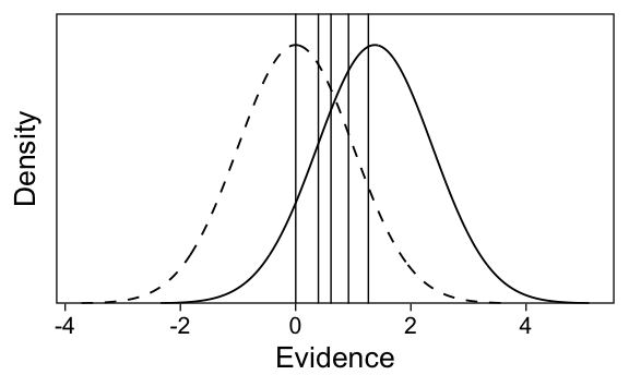
Figure 5: Signal detection model of participant 1’s rating data, visualized from the parameters’ posterior means. The two distributions are the noise distribution (dashed) and the signal distribution (solid). Vertical lines are the estimated thresholds. d’ is the distance between the peaks of the two distributions.
Model for multiple participants
For a sample of subjects, we could again compute each individual’s parameters and summarize them in another model. We won’t bother but instead turn immediately to a multilevel model formulation. A multilevel model, however, can take at least two forms. The first, shown now, includes subject-specific deviations in the linear model of \(\eta\):
Notice that we again omit any population-level intercept in Equation 7, but include by-subject random intercepts \(\gamma_0\). I omit expanding \(\Sigma\) here–it is the same as in Equation 4. The brms syntax is the same as in Listing 7, but instead of a bernoulli outcome distribution, we use cumulative() (Listing 9). Alternatively, the model syntax is identical to that in Listing 8, but we now include subject-specific random coefficients with (stimulus | pid).
Listing 9: Estimating a cumulative model for multiple participants with brm().
Draw your attention to the “Multilevel Hyperparameters” section. The standard deviation of the model intercept in the population is approximately 0.3 (posterior mean), and that of the d’ is ~0.5. However, the link function of the model partitions the latent normal (“evidence”) distribution into k (6) categories using k-1 thresholds (5). The latter are estimated for the population and shown above as Intercept[1-5]. Why is there only a standard deviation parameter for one intercept?
The answer, in brief, is that it is difficult to estimate subject-specific thresholds as random parameters and simultaneously retain their ordering. Therefore, the brms syntax estimates instead one “slope” parameter for each participant that shifts the entire evidence distribution for that participant, relative to the “average subject”. The interpretation of such a shift is interchangeably either that a participant’s evidence distribution has shifted, or that their thresholds have shifted by an identical amount. We agree with the latter interpretation—an equal shifting of the thresholds—because it makes little sense to assume that anyone would have a non-zero evidence distribution for noise stimuli.
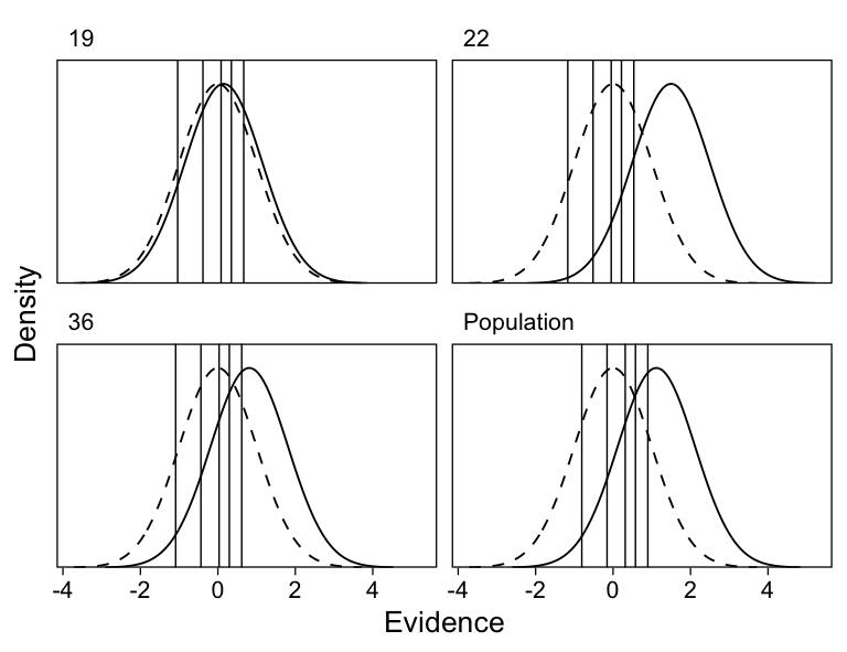
Figure 6: Implied SDT model from multilevel regression model with by-subject random intercepts and slopes. Density curves indicate latent evidence distributions (dashed line: noise trials; solid line: signal trials). Vertical lines indicate thresholds.
To aid interpretation, I have also visualized the multilevel cumulative model’s implied SDT model, for the population average and three subjects, in Figure 6. A close inspection of this figure reveals that the distance between the thresholds (vertical lines) is identical for every participant (and the population average). While this formulation of the model is parsimonius, it is important to note that it could be considered in violation of some SDT assumptions by not allowing these thresholds to flexibly vary between individuals. To address this potential limitation, we now estimate a variation of this model that estimates fixed subject-specific thresholds.
A multilevel model with subject-specific thresholds
The syntax for this model is similar to above, but we use thres(gr = pid) to specify that the thresholds should be estimated separately for each participant (Listing 10). Then, we omit subject-specific random intercepts by (0 + stimulus | pid) and cmc = FALSE, which ensures that R’s default cell-mean coding for models without an intercept is disabled. Finally, we increase the adapt_delta control parameter from its default 0.8 to better estimate the model’s posterior distribution.
Listing 10: Estimating multiple participants’ rating data with a cumulative model with fixed subject-specific thresholds.
This “fixed thresholds” model is conceptually very similar to the “random intercepts” model above, but instead of estimating one deviation per subject, we have estimated all five thresholds for all participants. To make this clear, I show the model’s summary below. Contrast this to summary above, which reported random intercepts (their SD as sd(Intercept)) and slopes (sd(stimulusOld)), this only includes random slopes and instead fixed (“population level”) thresholds for participants, reported as Intercept[subject, threshold], below:
Code
# Prevent printing too much informationmax_print <-getOption("max.print")options(max.print =35).summary(fit_evsdt_thresholds)
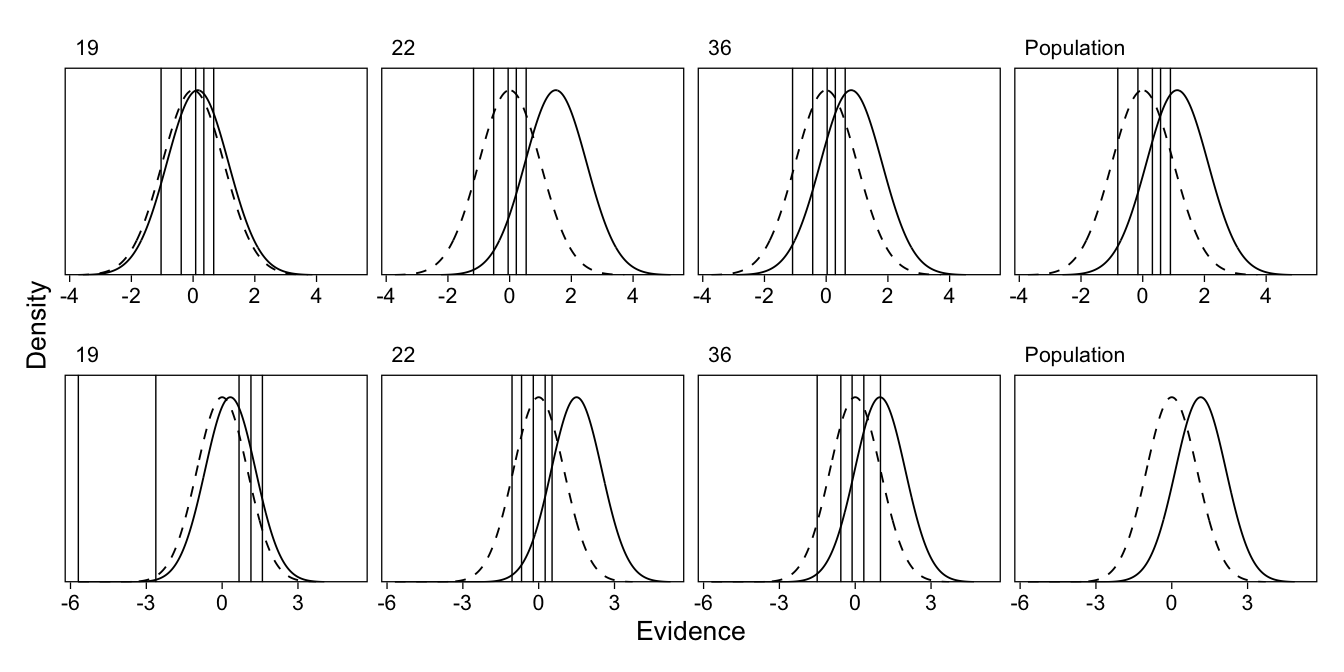
To help clarify the difference between these two models, I show the implied latent distributions and thresholds from the “fixed thresholds” model in Figure 7 (along with Figure 6). As is shown, the “fixed thresholds” model (bottom) allows for flexible thresholds for each participant, whereas the “random intercepts” model (top) only allows the average location of the thresholds to vary between participants. Also notable is the extremely low first threshold for participant 19: This participant had zero “1 (sure new)” responses (either for new or old items). Therefore the threshold location, when they are treated as fixed, not random, is completely decided by the prior distribution. By default, brms has used a \(t^+(3, 0, 2.5)\) prior.
Figure 7: Top. As Figure 6. Bottom. Implied SDT models for three participants, and population, from multilevel model with by-subject random slopes and fixed intercepts.
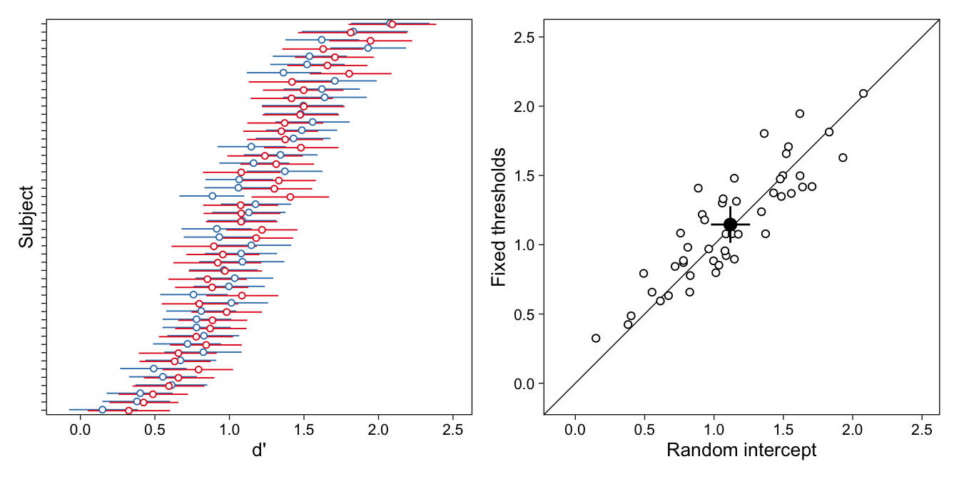
Given these two different models for essentially the same analytic problem, it is then critical to compare their key parameters. In Figure 8, I show d’s from both models for every participant. As shown, while the participant-specific parameters differ between models, the differences are small and their rank-orderings are very similar. Moreover, the population-level d’ is nearly identical between models.
Figure 8: Comparison of d’ parameters from multilevel rating model with random subject-specific intercepts (blue) and fixed subject-specific thresholds (red). Left. Posterior means and 95%CIs of d’ from both models; estimates are comparable and rank orders are reasonably similar. Right. Scatterplot of subject-specific d’ from the two models shows they are strongly correlated (r = [.80, .93]). Filled point and intervals indicate the population-level d’ and its 95%CI.
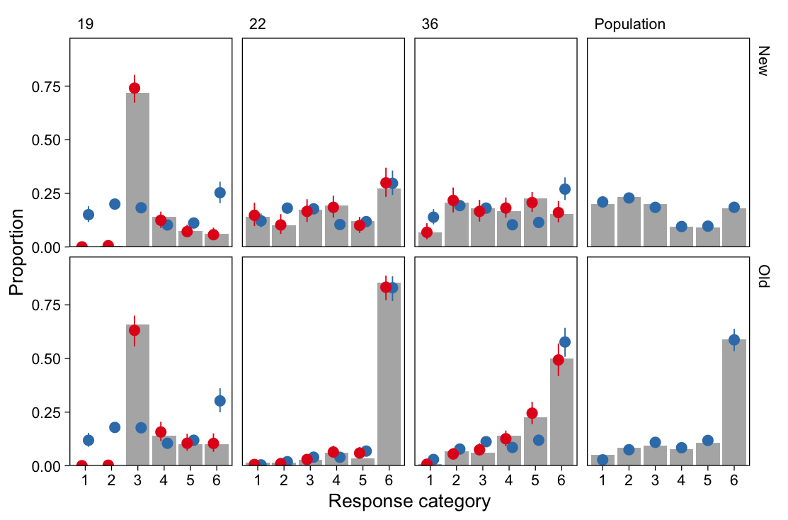
Finally, to conclude this diversion to the two different ways in which the SDT models for rating data can be estimated with regression for multiple subjects, Figure 9 shows the predicted proportions in each response category for three subjects, along with the values calculated from data. As shown, the model predictions are notably different for participant 19, who had no responses in the lowest category. The fixed thresholds model predicts this (lack of) data perfectly, whereas the random intercepts model overestimates the proportions. For participants with more well-behaved responses, the predictions are very similar.
Figure 9: Model-predicted response proportions from multilevel rating model with random subject-specific intercepts (blue) and fixed subject-specific thresholds (red), along with data (gray bars).
Moreover, Figure 9 reveals a critical difference between the models. The random-intercepts model is able to make predictions at the population level (which fit reasonably well), while the fixed thresholds does not. This is because the latter model does not estimate population-level thresholds, but instead its estimates are limited to the subjects in the current sample.
We now conclude the tutorial section on estimating basic signal detection theoretic models data using (multilevel) bayesian regression models, and turn toward more advanced SDT models.
Advanced SDT models
In this section, we cover the estimation of two generalizations of the SDT model, the unequal variances and finite mixtures models (for both single subjects and multiple individuals using multilevel regression). As above, our focus is on practical application; readers requiring a more theoretical treatment can refer to standard texts (Green and Swets 1966; Macmillan and Creelman 2005; Wickens 2001); a more complete mathematical treatment is DeCarlo (2010).
Unequal variances
The models discussed above have all assumed that the latent evidence distributions associated with signal and noise trials have the same variability. Accordingly, in more general treatments, the model above is known as the equal variance SDT (EVSDT) model. However, when tested, this assumption is consistently found inadequate: Experiments have repeatedly shown that the signal distribution has greater variance than the noise distribution in a wide variety of subject domains. For example, Koen et al. (2013) reported increased signal distribution variability across four memory experiments.
A generalization of the EVSDT model, the unequal variance (UVSDT) model adds one parameter to estimate the signal distribution’s variance. Recall that it is always assumed that the noise distribution has a standard deviation of 1. Importantly, we cannot estimate this additional parameter for binary outcomes (Yes/No task), and so below focus on the rating data.
The UVSDT model, for one participant’s data, is a generalization of Equation 5
This model—also knows as a probit model with heteroscedastic error (e.g. DeCarlo (2010))—can be readily estimated with the brms R package (Bürkner 2017; Bürkner and Vuorre 2019). Before we do so, we note that brms parameterizes this model with an equivalent formulation using different terminology, in line with conventions in item response theory (Bürkner 2021):
In this parameterization, \(\sigma = 1/\text{disc}\). We highlight this conversion below, when post-processing the model’s estimates. The brms syntax to estimate this model is similar to that of Listing 8, but we include an additional regression formula to predict disc. To do so, we wrap the main regression formula in bf() (used to predict the response distribution’s location parameter), and add a regression formula for disc using lf():
Listing 11: Estimating multiple participants’ rating data with an unequal variances cumulative model.
We print the model’s summary below. Before inspecting it in detail, refer to the model summary of the EVSDT model fitted to one subject’s rating data above. Notice that it reports an estimate of disc, which is fixed to one if no regression model for it is specified. Below, we obtain disc_stimulusOld, which is the discrimination parameter estimated from data.
For a standard SDT interpretation, it is then useful to post-process the model parameters to obtain an estimate of the signal distribution’s standard deviation (Listing 12).
Listing 12: Converting the log-discriminability parameter to a standard deviation.
From above, we find an estimated signal distribution standard deviation of approximately 1.24 (posterior mean). Plotting the model’s implied distributions illustrates this graphically (Figure 10).
Figure 10: The unequal variance Gaussian signal detection model, visualized from the parameters’ posterior means. The two distributions are the noise distribution (dashed) and the signal distribution (solid). Vertical lines are the thresholds, and d’ is indicated by the scaled distance between the peaks of the two distributions.
UVSDT for multiple participants
Above, we fit the UVSDT model for a single subject. However, we typically want to discuss inferences about the population, not individual subjects. Further, if we wish to discuss individual subjects, we should place them in the context of other subjects. A multilevel model accomplishes these goals by including both population- and subject-level parameters. We extend the code from Listing 11 to a hierarchical model by specifying varying parameters across participants Listing 13.
Recall from above that using |p| leads to estimating correlations among the varying effects. There will only be one standard deviation associated with the thresholds; that is, the model assumes that subjects vary around the mean threshold similarly for all thresholds. We can then estimate the model as before.
Listing 13: Estimating multiple participants’ rating data with an unequal variances cumulative model.
Let’s first focus on the Regression Coefficients: The effects for the “average person”. Intercepts, again, indicate the thresholds used to partition the latent evidence distribution into response categories. stimulusOld is d’, disc_stimulusOld is \(-\text{log}(\sigma_{signal})\). It is typically useful to transform the latter to a standard deviation, as is shown in Listing 12.
Mixture SDT model
While the unequal variances SDT model fits observer data better than does the equal variances model, it provides no explanation to why the latent variances might differ. One explanation for this difference is that observers might, on a subset of trials, be inattentive to the task:
An inattentive observer dozes off, or at least drifts into reverie, on some proportion of trials; because failing to respond is usually discouraged,this leads to an unknown numberof d′=0 trials,ones on which the observer responds despite not having paid attention, mixed in with the others (Macmillan and Creelman 2005, 46)
In this section, I briefly outline how the mixture SDT model discussed in DeCarlo (2010) can be fit with brms. Substituting \(\lambda\) in DeCarlo (2010) (eqn. 19, p. 309) with \(\theta\), in line with how brms labels it, we can write the model as a mixture of two cumulative models (Equation 10).
The above equation is a mixture of two processes. The main process includes a predictor (\(\eta\)) and thus allows for an effect of stimulus, and the second process omits the predictor: On inattention trials there can be no effect of the stimulus as it was not attended to. We translate this model to brms’ syntax in Listing 14. The key addition here is the inclusion of two response distributions (family = mixture(), nmix = 2), and the inclusion of stimulus predictor in modeling only the first of these.
Listing 14: Estimating a mixture SDT model for one participant.
I show results of this model below. First, although the summary reports two vectors of thresholds, one for each response distribution in the mixture, they are automatically constrained to equality (mu1_Intercept[1] = mu2_Intercept[1]; see ?mixture), as we wanted for this model. Second, mu1_stimulusOld is d’; the effect of stimulus for the first response distribution mu1—notice that there is no effect for the second distribution (mu2).
By default, this model has fixed the latent variances at 1 (disc1 = disc2 = 1). But now we have two additional parameters theta1 that index the mixture proportions. We see that participant 1’s responses are a mixture of ~86% attended trials, and ~14% non-attended trials (posterior means). For more details on interpreting this model, see DeCarlo (2010).
Multilevel mixture SDT model
After estimating the mixture model for one participant, we now turn to estimating it for a sample of individuals using a multilevel model. The syntax (Listing 15) is identical to that in Listing 14, but we now include by-person random effects on the parameters.
Listing 15: Estimating a mixture SDT model for multiple participants with a multilevel model.
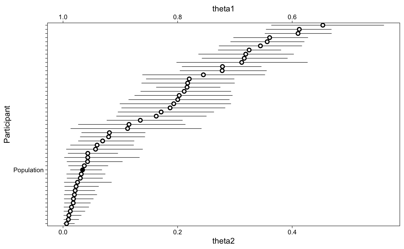
I print the summary of this model’s results below. In addition to Multilevel Hyperparameters (the parameters’ heterogeneities in the population), we now have an estimate of the average mixing proportion of the second component theta2_Intercept, but this is reported on scale of the link function (logits).
Therefore, we transform the population-level and individual-specific mixture proportions from the logit space to proportions, and then display the estimates in Figure 11.
Figure 11: Mixing proportions for each participant (empty) and the population (filled).
Conclusion
Signal Detection Theory is “one of the greatest successes of mathematical psychology” (Wickens 2001). It is used to guide theorizing and data analyses in a wide variety of research areas in psychology where the experimental tasks involve detecting, or indicating one’s confidence in, the presence of a signal. Those “signals” can be previously seen images or words, perceptual stimuli corrupted by noise, marks of illness, and more. The theory itself is established and further made accessible in widely read texts (Green and Swets 1966; Macmillan and Creelman 2005).
While many SDT models are accessible to researchers via well-known computational formulas (Stanislaw and Todorov 1999), those don’t always easily generalize to more complex research designs, and can ignore important sources of variability (e.g. due to item heterogeneity Rouder and Lu 2005; see also Rouder et al. 2007). Moreover, these calculations introduce added complexity to researchers, who do not always recognize that the models can be estimated with standard tools, such as Generalized Linear (Mixed) Models [GLMM; DeCarlo (1998); Decarlo (2003)] that are straightforward to generalize to more complex research designs.
My aim with this tutorial was to provide an introduction to how the GLMM can be used to estimate a variety of SDT models, ranging from single-subject analyses to multilevel mixture models that account for attention lapses, using bayesian regression methods implemented in the brms R package (R Core Team 2025; Bürkner 2017).
References
Bolger, Niall, and Jean-Philippe Laurenceau. 2013. Intensive Longitudinal Methods: An Introduction to Diary and Experience Sampling Research. Guilford Press. http://www.intensivelongitudinal.com/.
Bürkner, Paul-Christian. 2017. “Brms: An R Package for Bayesian Multilevel Models Using Stan.”Journal of Statistical Software 80 (1): 1–28. https://doi.org/10.18637/jss.v080.i01.
Bürkner, Paul-Christian. 2021. “Bayesian Item Response Modeling in R with Brms and Stan.”Journal of Statistical Software 100 (November): 1–54. https://doi.org/10.18637/jss.v100.i05.
Bürkner, Paul-Christian, and Matti Vuorre. 2019. “Ordinal Regression Models in Psychology: A Tutorial.”Advances in Methods and Practices in Psychological Science 2 (1): 77–101. https://doi.org/10.1177/2515245918823199.
Cohen, Andrew L., Jeffrey J. Starns, and Caren M. Rotello. 2021. “Sdtlu: An R Package for the Signal Detection Analysis of Eyewitness Lineup Data.”Behavior Research Methods 53 (1): 278–300. https://doi.org/10.3758/s13428-020-01402-7.
Decarlo, Lawrence T. 2003. “Using the PLUM Procedure of SPSS to Fit Unequal Variance and Generalized Signal Detection Models.”Behavior Research Methods, Instruments, & Computers 35 (1): 49–56. https://doi.org/10.3758/BF03195496.
DeCarlo, Lawrence T. 2010. “On the Statistical and Theoretical Basis of Signal Detection Theory and Extensions: Unequal Variance, Random Coefficient, and Mixture Models.”Journal of Mathematical Psychology 54 (3): 304–13. https://doi.org/10.1016/j.jmp.2010.01.001.
Gelman, Andrew, John B. Carlin, Hal S. Stern, David B. Dunson, Aki Vehtari, and Donald B. Rubin. 2013. Bayesian Data Analysis, Third Edition. Chapman; Hall/CRC.
Gelman, Andrew, and Jennifer Hill. 2007. Data Analysis Using Regression and Multilevel/Hierarchical Models. Cambridge University Press. http://www.stat.columbia.edu/~gelman/arm/.
Kellen, David, Samuel Winiger, John C. Dunn, and Henrik Singmann. 2021. “Testing the Foundations of Signal Detection Theory in Recognition Memory.”Psychological Review 128 (6): 1022–50. https://doi.org/10.1037/rev0000288.
Koen, Joshua D., Mariam Aly, Wei-Chun Wang, and Andrew P. Yonelinas. 2013. “Examining the Causes of Memory Strength Variability: Recollection, Attention Failure, or Encoding Variability?”Journal of Experimental Psychology: Learning, Memory, and Cognition 39 (6): 1726–41. https://doi.org/10.1037/a0033671.
Kruschke, John K. 2014. Doing Bayesian Data Analysis: A Tutorial Introduction with r. 2nd Edition. Academic Press.
Kruschke, John K., and Torrin M. Liddell. 2017a. “Bayesian Data Analysis for Newcomers.”Psychonomic Bulletin & Review, April 12, 1–23. https://doi.org/10.3758/s13423-017-1272-1.
Kruschke, John K., and Torrin M. Liddell. 2017b. “The Bayesian New Statistics: Hypothesis Testing, Estimation, Meta-Analysis, and Power Analysis from a Bayesian Perspective.”Psychonomic Bulletin & Review, February 7, 1–29. https://doi.org/10.3758/s13423-016-1221-4.
Lee, Michael D. 2008. “BayesSDT: Software for Bayesian Inference with Signal Detection Theory.”Behavior Research Methods 40 (2): 450–56. https://doi.org/10.3758/BRM.40.2.450.
Leeuwen, Florian van, Bastian Jaeger, John Axelsson, et al. 2024. “The Smoke-Detector Principle of Pathogen Avoidance: A Test of How the Behavioral Immune System Gives Rise to Prejudice (Stage 1 Registered Report).” Pre-published September 30. https://doi.org/10.31234/osf.io/e874s.
Licklider, J. C. R. 1959. “Three Auditory Theories.” In Psychology: A Study Of A Science Volume, edited by Sigmund Koch, 1: Sensory Perceptual And Physiological Formulations. McGraw-Hill. https://archive.org/details/in.ernet.dli.2015.74438.
Liddell, Torrin M., and John K. Kruschke. 2018. “Analyzing Ordinal Data with Metric Models: What Could Possibly Go Wrong?”Journal of Experimental Social Psychology 79 (November): 328–48. https://doi.org/10.1016/j.jesp.2018.08.009.
Macmillan, Neil A., and C. Douglas Creelman. 2005. Detection Theory: A User’s Guide. 2nd ed. Lawrence Erlbaum Associates.
McElreath, Richard. 2020. Statistical Rethinking: A Bayesian Course with Examples in R and Stan. 2nd ed. CRC Texts in Statistical Science. Taylor and Francis, CRC Press. https://xcelab.net/rm/statistical-rethinking/.
Paulewicz, Borysław, and Agata Blaut. 2020. “The Bhsdtr Package: A General-Purpose Method of Bayesian Inference for Signal Detection Theory Models.”Behavior Research Methods 52 (5): 2122–41. https://doi.org/10.3758/s13428-020-01370-y.
R Core Team. 2025. R: A Language and Environment for Statistical Computing. Version 4.4.3. V. 4.4.3. R Foundation for Statistical Computing, released. https://www.R-project.org/.
Rouder, Jeffrey N., and Jun Lu. 2005. “An Introduction to Bayesian Hierarchical Models with an Application in the Theory of Signal Detection.”Psychonomic Bulletin & Review 12 (4): 573–604. https://doi.org/10.3758/BF03196750.
Rouder, Jeffrey N., Jun Lu, Dongchu Sun, Paul Speckman, Richard D. Morey, and Moshe Naveh-Benjamin. 2007. “Signal Detection Models with Random Participant and Item Effects.”Psychometrika 72 (4): 621–42. https://doi.org/10.1007/s11336-005-1350-6.
Singmann, Henrik, and David Kellen. 2013. “MPTinR: Analysis of Multinomial Processing Tree Models in R.”Behavior Research Methods 45 (2): 560–75. https://doi.org/10.3758/s13428-012-0259-0.
Stanislaw, Harold, and Natasha Todorov. 1999. “Calculation of Signal Detection Theory Measures.”Behavior Research Methods, Instruments, & Computers 31 (1): 137–49. http://link.springer.com/article/10.3758/BF03207704.
Vuorre, Matti, Matthew Kay, and Niall Bolger. 2024. “Communicating Causal Effect Heterogeneity.” Pre-published September 3. https://doi.org/10.31234/osf.io/mwg4f.
Zloteanu, Mircea, and Matti Vuorre. 2024. “A Tutorial for Deception Detection Analysis or: How I Learned to Stop Aggregating Veracity Judgments and Embraced Signal Detection Theory Mixed Models.”Journal of Nonverbal Behavior, ahead of print, March 1. https://doi.org/10.1007/s10919-024-00456-x.
Appendices
Additional SDT metrics
Above, we discussed the common SDT metrics c and d’ that index a respondent’s bias and sensitivity, respectively. Here, we discuss some additional metrics that are commonly used in the SDT literature. The hit and false alarm rates, and their corresponding z-scores, are used in the manual calculation of these metrics, but can be useful in their own right. From the modeling perspective, these rates are outcomes, and we can therefore use methods to predict them from the model. In Listing 16, we use functions from the tidybayes package (Kay 2024). I show the results of these calculations in Table 7.
Listing 16: Calculate predicted rates from a single subject’s model.
Code
# Predict outcomes for these predictorsx <-tibble(stimulus =c("New", "Old"))# Predicted ratesrates <-epred_draws(fit_glm, x, value ="rate") |>mean_qi()# Predicted z-scored ratesz_rates <-linpred_draws(fit_glm, x, value ="rate") |>mean_qi()
Table 7: Model-predicted hit (stimulus=Old) and false alarm (stimulus=New) rates of responding ‘Old’.
Type
stimulus
rate
.lower
.upper
Rates
New
0.27
0.20
0.34
Rates
Old
0.77
0.70
0.84
zRates
New
-0.62
-0.84
-0.42
zRates
Old
0.75
0.52
0.98
Including predictors
Do the EVSDT parameters differ between groups of people? How about between conditions, within people? To answer these questions, we would repeat the manual calculation of parameters as many times as needed, and then draw inference by “submitting” the subject-specific parameters to e.g. an ANOVA model. The GLMM approach affords a more straightforward solution to including predictors: We simply add parameters to the regression model.
For example, if there were two groups of participants, indexed by variable group in data, we could extend the brms GLMM syntax to:
brm(response ~ stimulus * group + (stimulus | pid), ...)
This model would have two additional parameters: group would describe the difference in c between groups, and the interaction term stimulus:group would describe the difference in d’ between groups. If we were additionally interested in the effects of condition, a within-subject manipulation, we could write:
The Receiving Operator Characteristic (ROC) curve displays hits as a function of false alarms, for possibly multiple criteria, and is a useful description of detection data in its own right. As such, it is useful to be able to generate ROC curves implied by the model. Here, we illustrate how to obtain ROC curves from fitted models with uncertainty estimates and overlay them on raw data.
First, I show code for calculating (z-scored) hit and false alarm rates both from data, and as predicted from the multilevel equal variances cumulative model (Listing 17).
Listing 17: Calculating (z-scored) hit and false alarm rates from data and model predictions, at the population level and that of individual subjects.
Code
# Population level ratesroc_dat <-left_join(# From model (posterior means) dat2 |>distinct(stimulus) |>add_epred_draws(fit_evsdt, re_formula =NA) |>mean_qi() |>mutate(response =as.integer(.category),pid ="Population" ) |>select(pid, stimulus, response, .epred),# From data dat2 |>summarise(pid ="Population",n =sum(n),.by =c(stimulus, response) ) |>mutate(p = n /sum(n), .by = stimulus),by =c("pid", "stimulus", "response"))# Subject-level ratesroc_sub <-left_join(# From model dat2 |>distinct(pid, stimulus) |>add_epred_draws(fit_evsdt) |>mean_qi() |>mutate(response =as.integer(.category)) |>select(pid, stimulus, response, .epred),# From data dat2 |>summarise(n =sum(n),.by =c(pid, stimulus, response) ) |>mutate(p = n /sum(n), .by =c(pid, stimulus)),by =c("pid", "stimulus", "response"))# Combine population- and subject level data, and calculate cumulative ratesroc_dat <-bind_rows( roc_dat, roc_sub) |>select(-n) |>pivot_longer(c(.epred, p)) |>pivot_wider(names_from = stimulus, values_from = value) |># Cumulate proportions from high to low response categoryarrange(pid, desc(response)) |>mutate(hr =cumsum(Old),fr =cumsum(New),zhr =qnorm(hr),zfr =qnorm(fr),.by =c(pid, name) )
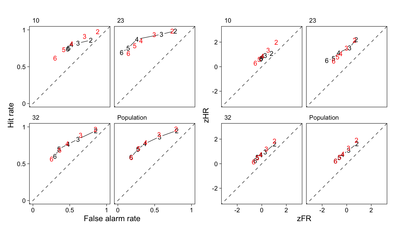
Having calculated the hit and false alarm rates in both their natural and probit scales, all that is left to do is to plot them. In Figure 12, we show these rates for a sample of participants, and the population. While interpreting these figures, it is important to keep in mind that the data-based coordinates have error in both the x- and y-axes.
Figure 12: Receiver operating characteristic plots in the proportion (left) and z-score scales (right) for three participants and the population. Black symbols and lines are coordinates calculated from data, red symbols are model-predicted rates.
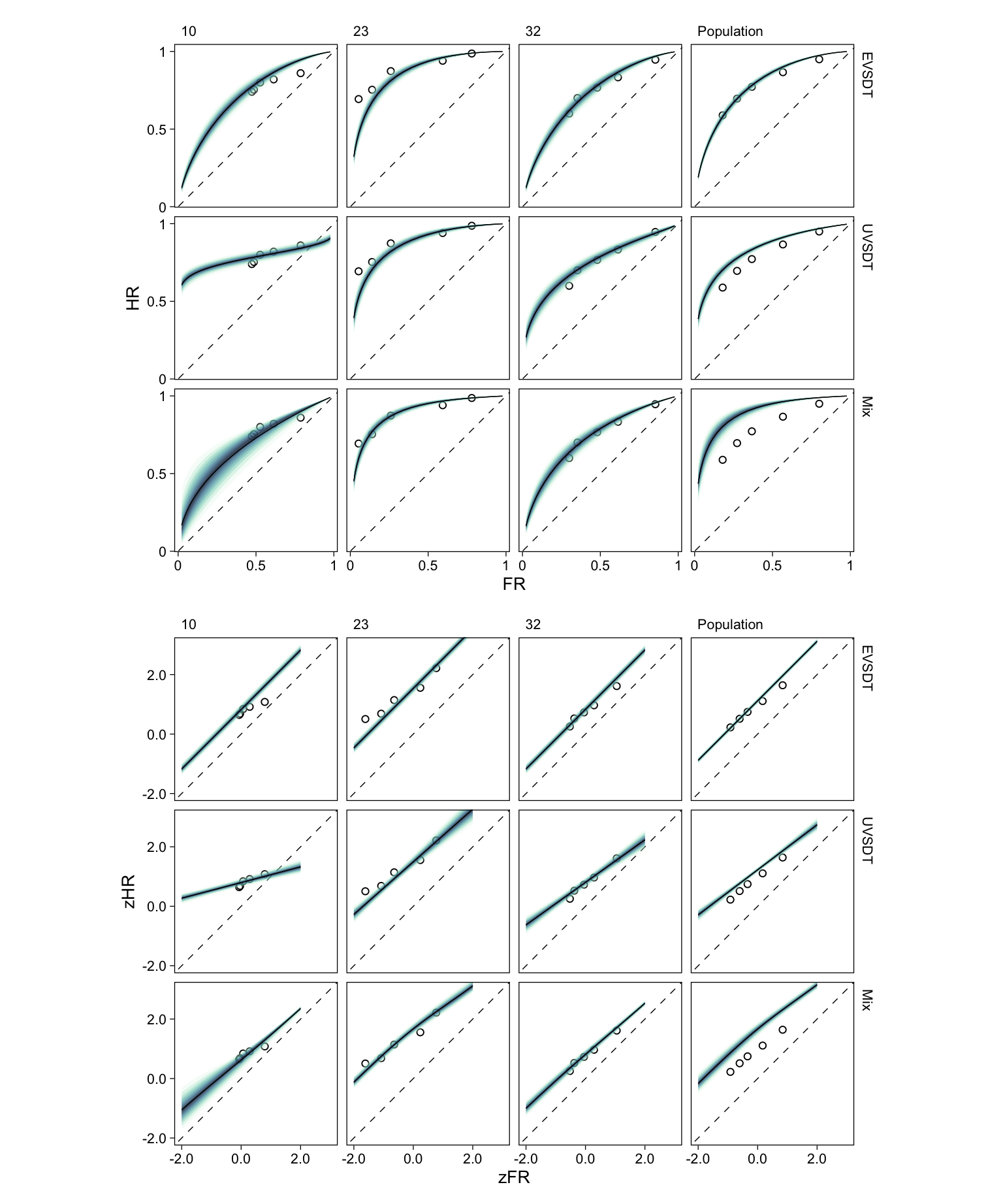
Next, we draw a more complete picture by using the model to predict (z-scored) hit rates for the entire range of hypothetical false alarm rates. We obtain the predicted ROC curves from the multilevel EVSDT, UVSDT, and mixture models at both the population- and participant-specific levels.
Listing 18: Calculating predicted ROC curves from multilevel EVSDT, UVSDT, and mixture models.
Above, we made use of the file argument in brm() to save estimated models to a file. Throughout, I have also used other options to speed up sampling, specified in a special .Renviron file:
# Contents of .RenvironMAX_CORES=8BRMS_BACKEND="cmdstanr"BRMS_THREADS=2
With these settings, every call to brm() uses the variables I have specified in .Renviron to speed up model estimation with values that work well on my local machine (that has eight CPU cores.) For more information, see ?brm and ?Sys.getenv.
@misc{vuorre2017,
  author = {Vuorre, Matti},
  title = {Estimating {Signal} {Detection} {Models} with Regression
    Using the Brms {R} Package},
  date = {2017-10-09},
  url = {https://osf.io/preprints/psyarxiv/vtfc3_v1},
  doi = {10.31234/osf.io/vtfc3_v1},
  langid = {en},
  abstract = {Signal Detection Theory is a widely used framework for
    understanding decisions by distinguishing between response bias and
    true discriminability in various psychological domains. Manual
    calculation approaches to estimating SDT models’ parameters, while
    commonly used, can be cumbersome and limited. In this tutorial I
    connect SDT to regression models that researchers are already
    familiar with in order to bring the flexibility of modern regression
    techniques to modeling of SDT data. I begin with a glance at SDT’s
    fundamentals, and then show how to manually calculate basic SDT
    parameters. In the bulk of the tutorial, I show step-by-step
    implementations of various SDT models using the brms R package. I
    progress from analyses of binary Yes/No tasks to rating task models
    with multilevel structures, unequal variances, and mixtures.
    Throughout, I highlight benefits of the regression-based approach,
    such as dealing with missing data, multilevel structures, and
    quantifying uncertainty. By framing SDT models as regressions,
    researchers gain access to a powerful set of flexible tools while
    maintaining the conceptual clarity that makes SDT valuable. A
    regression-based approach not only simplifies SDT analyses but also
    extends SDT’s utility through flexible parameter estimation with
    uncertainty measures and the ability to incorporate predictors at
    multiple levels of analysis.}
}
For attribution, please cite this work as:
Vuorre, Matti. 2017. “Estimating Signal Detection Models with
Regression Using the Brms R Package.” In PsyArXiv.
Preprint, October 9. https://doi.org/10.31234/osf.io/vtfc3_v1.